Role of "R Squared Change" in Multiple Regression Analysis (MRA)

R.W. writes, "In the PowerPoint walk through for Research Design Forum #3 (RDF3), at the point of the MRA configuration, you did not specify to check the "R squared change" box. It shows the statistics in the next slide and references to it, but I am not sure if it is really needed to complete the assignment. I wanted to let you know in case there was any confusion for others when doing the discussion post."

You raise a good question. MRA is largely concerned with identifying the amount of explained variation in the dependent variable (Y) from the linear contributions of all independent and control variables selected for inclusion in the equation on a range from 0 to 100 percent. The statistic that reveals this explained variation is R-Squared (R2), i.e., the multiple correlation coefficient (R) squared. Your question centers on how the researcher wants those Xs and control variables introduced into the regression model - forward, backward, stepwise, forced entry as a block, etc. This decision will depend on what is hoped to be accomplished through the MRA by the researcher.

Often there is a theoretical interest in first introducing/regressing a key independent variable (X1) in the regression model, via the main hypothesis, and assessing the simple regression output (i.e., the beta, R and R2). Here, the identified beta (a regression coefficient) and R (a multiple correlation coefficient) both equal the Pearson’s r (a zero-order correlation coefficient) between that X1 and Y since there’s only one independent variable in the equation. As I mentioned above, R2 provides the amount of explained variation in Y from X1 on a range from 0 percent to 100 percent. Armed with this important bivariate statistical information, the researcher can then move to expand or elaborate on the hypothesized bivariate relationship by adding key independent and control variables that are theoretically relevant to the research and then selecting the R-Squared Change option. This procedure will allow the researcher to identify change in the original R2 (as well as X1’s beta) based on the linear contribution of variables added into the regression model when those additonal variables are held constant. Note that the significance of the total equation can only be found through the F statistic and its level of significance as measured by the p value (conventionally, p must be < .05).  The F statistic and its level of significance (via the p value) also appear in the regression output.

In short, to your question and the class assignment, all variables were “forced” into the equation at once using the default METHOD=ENTER option. In this case, Robert, there is no R Squared Change to be reported. If we ran a different MRA method, such as that described above, then the "R-Squared Change" option would be appropriate and highly useful.

I hope this helps!

Professor Ziner

SPSS/PASW 18 Core System and Statistics User’s Guides are Available to Download

There are many important reasons for obtaining a user’s guide for software packages. The least of which is to be able to identify and access each available software option and, once accessed, understand exactly how to “put it to use” in practice. This is especially true when opening the Statistical Package for the Social Sciences or SPSS (now rebranded by IBM as PASW).  SPSS helps researchers to address a series of unavoidable challenges when they conduct quantitative research (e.g., How to: build a versatile database, enter and define data, transform/recode variables, merge external data into an existing data set, run a series of statistical tests, generate tables and charts, develop reports, and so on). The problem is that student researchers often have both procedural and data analysis-oriented questions about SPSS that often occur outside of the time spent conducting in-class SPSS assignments.

To address this concern, the SPSS/PASW 18 Core System User's Guide and SPSS/PASW 18 Statistics Base User’s Guide are now available for you to download to your hard drive. The documents range from 3-5MB so be sure you have a little time to download them if your internet access is not high speed. There are two ways to access each user’s guide:

1. Locate “SPSS 18 User’s Guides” on the left side of Broken Pencils, right-click over the User's Guide of interest, click on SAVE TARGET AS and save it to the location of your choice (such as your hard drive or a flash drive).
2. Right-click on this link: SPSS 18 Core System User’s Guide, click on SAVE TARGET AS and save it to the location of your choice.
3. Right-click on this link: SPSS 18 Statistics Base User’s Guide, click on SAVE TARGET AS and save it to the location of your choice.

Once they're downloaded, be sure to put them in a location that is easily accessible. When you open a user's guide in Adobe Reader (i.e., in .pdf format), use the tree structure on the left side of the screen to scroll down to the procedure you want explained. Did you forget how to RECODE a variable into a new one?  Just open the SPSS/PASW 18 Core System User's Guide, scroll down to Data Transformations (CH8), click on the RECODE sections and apply the procedure to your current needs.

Note: I have also provided the SPSS/PASW 18 Brief Guide on this site's menu of SPSS user's guides. This document usually accompanies the SPSS Student Version of the software program so, while it is more limited in scope, it can provide you with quick answers to your SPSS-based research needs.

I hope these documents are helpful.

Professor Ziner

How To Study Statistics

Since the outset of the term, I have been contacted by many students who seem to be asking the same question: “How do I study for your class?”  Relax.  All of you are not alone.  Many students have trouble learning statistics because they never develop the particular study habits which are conducive to success in my statistics classes. If you pay close attention to the following suggestions they should prove invaluable to you.

1. READ CAREFULLY AND DELIBERATELY. The way in which you should read in statistics is quite different from the way you may read a history book, newspaper, or a novel. In statistics you must read slowly, absorbing each word. It is sometimes necessary to read a textbook discussion or problem many times before it begins to "make sense" to you. In some types of reading, such as a novel, it is desirable to skim and read rapidly, because there are usually a few thoughts "sprinkled" among many words. However, in reading statistics each word or symbol is important because there are many thoughts condensed into a few statements. Keep in mind that the little words mean a lot in statistics.
   
   
2. THINK WITH PENCIL AND SCRATCH PAPER. Always have pencil in hand and scratch paper ready and use them when you read and study statistics. Test out the ideas on paper that the authors are discussing. When they propose a question, try to answer it before going on. Even though an example may be worked out completely in the text, work it out for yourself on scratch paper. This will help to clinch the ideas and procedures in your mind before starting the exercises. After you have read and reread a problem carefully, if you still don't see what to do, don't just sit and look at it. Get your pencil going on scratch paper and try to "dig it out.” If, in attempting to solve a problem, you have nothing written on paper, then you have not yet exerted enough effort to justify seeking help.
   
   
3. BE INDEPENDENT. Try to complete each lesson without assistance. If you seek help needlessly, either from me, a classmate, this Broken Pencils’ blog, or a math tutor, you will not gain the maximum benefit from your work. It takes exercise, as you know, to become strong.  You cannot learn statistics through someone else's exercise.  However, you must ask questions when necessary.  That’s what this blog is for.  Sometimes little things cause considerable confusion. Do not be afraid that your question may sound "dumb."  The only "dumb" action is to fail to ask about a topic that you have really tried to grasp and still do not get.  Some people seek help too soon and some wait too long.  You will have to use good common sense in this matter.
   
   
4. LISTEN IN CLASS AND READ MY BLOG (Broken Pencils).  Many of the finer points, fundamental principles and modes of thought will be developed in class.  You must pay careful attention to these educational objectives to really understand what is going on.  Take notes!  Also, many of these points are (or will be) available at this course blog. Join it to receive notification of new posts in your in-box as soon as they are posted.  I’ve already had students ask basic questions that would have been fully addressed if they tuned into the blog.  Note that Broken Pencils is growing weekly (first launched on 8/28/2010), so join to receive updates and benefit from the discussion.
   
   

How to Find the Upper and Lower Limits of Class Intervals

J.D. asked about the way statisticians identify upper and lower limits of class intervals found in a variable's frequency distribution.  When data are comprised of interval/ratio numbers or class intervals, e.g., (20-29) (30-39) (40-49) and so on, the limits of such numbers or class intervals are understood in terms of “true (real) limits.”  True/real limits are defined by the highest possible value – the upper limit – and the lowest possible value – the lower limit. The general rules for calculating the true limits of class intervals represented by numbers are:

Upper True Limit:  Add a 5 to the decimal place to the right of the last number appearing in the highest value specified by the number in the class interval.

Lower True Limit:  Subtract a 5 to the decimal place to the right of the last number appearing in the lowest value specified by the number in the class interval.

If the class intervals of a variable are defined by whole numbers, to find the upper limit we add .5 to the highest value specified by the category, and to find the lower limit we subtract .5 from the lowest value specified in the category.  The limits of other numbers could be similarly determined.  The table below provides some illustrations.

Click to Enlarge

Exporting SPSS Graphs and Tables

After generating output in SPSS and deciding to export some of the charts and tables into MS Word, several students found that some tables "don't quite fit" the (default) margins of the page. In this brief discussion, you will learn to export output (e.g., graphs and tables) from SPSS into Microsoft Word and other programs such as PowerPoint.

Procedure

You can export a graph or table by right clicking to bring up a pop-up menu. You have several choices in how to save the file and how to import it into another software program. While there are many choices, I have found that exporting tables and graphs into a Microsoft Word (.doc) format works well. Use of the .pdf format may be a bit premature, since statistical  output represent the building blocks of analysis and report writing in various word-processing and presentation software -- not the final product. You are encouraged to experiment with alternatives to see what best meets your needs.

Once a statistical procedure is performed in SPSS, we'll need to export a table, chart or text into MS Word so the output can be analyzed and a report developed. Just right-click over the object(s) -- a chart or table -- you want to export. An "Export Output" window will appear (see inset image below). The default format, Word/RTF (.doc), is likely the best format for course-based assignments.

Click to Enlarge

Under "File Name," you can determine where the Word/RTF document will be located, including a specific subdirectory on your hard drive or flash drive or to disc.  From within the newly saved document, you can change the appearance of the table, including altering its color, font style, size and direction and many more options.  Word interprets each SPSS table in ways similar to when you create your own within the program.  Just highlight an imported table and the "DESIGN" tab among Word's Table Tools appears.  It's your choice from there.

Sizing your Chart in MS Word

You may find an imported table or chart is wider than the margins in your document.  To address this, in the Word document, go to the "layout" portion, click "cell size" and then follow the chart below to make the chart shink to the size of a page.  This feature addresses the width of the output object.

Another way to shrink a table to make it fit better is to click to highlight a table in WORD and then click to single space it. Single spacing is found under the paragraph option in the HOME ribbon in MS Word.  You'll see the table shrink in height.

Happy Exporting!

Properties of Data in Statistical Analysis: Three Levels of Measurement (Nominal, Ordinal and Interval/Ratio)

S.B. asked me to comment on what are the “levels of measurement” I have been referring to in class, and importantly, what they have to do with our statistical forums conducted using SPSS. Good question, grasshopper. Let me try to put it in perspective.

So you plan to conduct a statistical analysis on a dependent variable (Y) and several independent variables (Xs) in your statistical forum due shortly. Where do you start? To be able to determine what statistical test is most appropriate for your task at hand, first you must assign a level of measurement to your study’s dependent variable: nominal, ordinal or interval/ratio. Your choice will depend on the type of variable that’s involved in your analysis. You should keep in mind that not only are variables measured differently but many variables can be measured at more than one level (see “Note” at the end of Pros and Cons to a Univariate Analysis). Although levels of measurement differ in many ways, they have certain similarities as well and can be classified using a few basic principles.

What do I mean by “measurement”?  Here are a few orienting points:

• Measurement can be defined as the assignment of numbers to a variable according to sets of predetermined rules
• The things we observe (gender or race, e.g.) are variables; any particular observation of that variable is an assigned number (e.g., "1" = male)
• We view the property of numbers that define the values of a variable

Here are the three fundamentally different ways in which numbers are used in statistical research:

1. Nominal Level Data: To name or identify
2. Ordinal Level Data: To represent position in a series or scale
3. Interval/Ratio: To represent quantity

Data Measured at the Nominal Level

When measuring a variable at the nominal level, the properties of the variables you’re working are categories. A number is then assigned to each category (e.g., for the variable “sex,” 1=male and 2=female). Race, region, and religion are additional examples of the numerous variables measured at the nominal level (sometimes referred to as the nominal scale). The main principle underlying nominal data is that they do not imply any ordering among the responses. Using “Party Affiliation" as an example (see inset chart below), the value of “1” for Republican is no more or less of the property of party affiliation than the value of "2" for Independent or “3” for Democrat. These numeric values are simply categories of the variable “Party Affiliation.” Data measured at the nominal level represent the lowest level of measurement.

Principles of Nominal Data: If the measurement tells only what class a case (e.g., a person) falls into with respect to the variable. Categories of nominal data are mutually exclusive and exhaustive.

Examples of Nominal Data:

1. Are you: __ (1) Male __ (2) Female
2. Are you: __ (1) Protestant __ (2) Catholic __ (3) Jewish __ (4) Muslim __ (5) Other

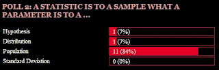
Second Class Poll Ends: A Statistic is to a Sample what a Parameter is to a Population

I’m not surprised that most (84%) who participated in the second class poll got it right (see the inset chart below). Over the first few class periods, my focus was to link the following four concepts: statistic, sample, parameter and population. Any discussion in a statistics class begins with this conceptual framework.

Since we seldom have complete knowledge of the parameters of a population, such as the mean of the population (µ) and its standard deviation (σ), we must obtain a representative (aka, random) sample from that population. In doing so, we are then working with statistics that describe the sample, not the population. Statistics calculated from sample data will, in turn, serve two broad purposes:

1. Descriptive Analysis. There are four ways that statistics describe sample data. They allow the researcher to examine levels of skewedness (degree of symmetry) and kurtosis (level of peakedness) of a variable’s distribution. They also quantify the central tendency (mode, median and mean) and dispersion (range, standard deviation and variance) of sample data that comprise a variable’s distribution.  Refer to my "Weekly PowerPoints" for details on the role of descriptive statistics.

2. Inferential Analysis. An important second purpose of sample statistics is to generalize outcomes found in sample data to the population from which the sample was drawn. The two broad roles for inferential analyses were reviewed in a previous blog which examined the outcome of our first class poll: Estimating Population Parameters and Testing Hypotheses.

The upshot is that for every statistic that describes some characteristic of a sample there is a corresponding parameter that describes the same characteristic of a population. We analyze sample statistics so that we may generalize statistical outcomes from the sample to the population of interest.

First Class Poll Ends: Inferential Analysis Involves …

The results of our first class poll (see inset chart below) reveal that most who participated correctly identified inferential analysis to involve two important forms of statistical research. The first is that we estimate population (N) parameters. Parameters describe populations of interest and include the mean of the population (µ) and its standard deviation (σ). Since researchers do not always know these characteristics of a population under study, they must be estimated from sample data. In the case of µ, we calculate confidence intervals (usually based on 95% or

99% confidence) to assess the range within which a true population parameter will fall. If you provided a single estimate of 190 lbs. for my weight, for example, how confident would you be that it’s correct? If you then widened your point estimate to an interval estimate of 180-200 lbs., wouldn’t you be more confident that my true weight is in this range? How about 160-220 lbs.? The point is that the wider the interval, the greater our confidence that the true µ falls within that interval.

Second, inferential analysis also involves hypothesis testing — a building block of research. A hypothesis is a statement of the relationship between two (or more) variables where one is seen as the independent variable (symbolized as X or the “cause”) and the other is the dependent variable (symbolized as Y or the “effect”). What is the effect of cigarette smoking (X) on rates of cancer (Y)? Hours studying statistics (X) on course grade performance (Y)? Size of a company (X) and employee job satisfaction (Y)? When we are interested in determining the statistical significance of these relationships by testing the effects of one variable on the other, we test hypotheses. Note that we cannot determine causality through hypothesis testing alone. Causality involves demonstrating statistical covariation and determining time-order (via variable manipulation procedures) and establishing statistical control (removing the possibility that some third factor can explain away X and Y’s significant covariation). Of the three elements of causality (covariation, manipulation and control), hypothesis testing provides the means to demonstrate statistical covariation of a bivariate (two-variable or "X on Y") relationship – an important first step in understanding and explaining the world around us.

The last two choices, “Generalizing to Samples” and “Heavy Drinking on Weekends,” are simply wrong. While conducting inferential analysis may lead some people to drink heavily on weekends (an interesting study in its own right), the process does not involve such behavior any day of the week.

I encourage you to participate in future class polls found at Broken Pencils! I will always analyze the results when the polling period expires and examine the answers to the questions I pose.

NOTE: Percentages do not add up to 100. This poll gave students the option of choosing more than one response. Future polls will be limited to one choice.

Pros and Cons to a Univariate Analysis

One purpose of our SPSS statistics forums is to effectively communicate quantitative information about sample data to your audience (e.g., your client, boss or, in your case, professor). We have already discussed how studies conducted on sample data involve a combination of descriptive and inferential statistics. The first task of a researcher is to examine what has been collected using one or more descriptive statistics. Often referred to as a “univariate” (one-variable) analysis, the goal is to describe each variable of interest in your database using the best possible statistic(s). The usual suspects include measures of central tendency (mean, median and mode) and dispersion (range and standard deviation). To visually display the distribution of a variable, a percentage distribution, bar chart or histogram is useful. The question is whether the descriptive statistics chosen fit the level of measurement that characterizes a variable (i.e., whether X or Y is nominal, ordinal or interval/ratio). For example, if you create the variable “sex” using 1=male and 2=female in SPSS, reporting its mean would be meaningless (a mean of 1.5 tells us what?). Consequently, the only useful statistic is the frequency or percentage of each sex in the sample (e.g., 60 percent of the sample were female). If you want, you can add a bar chart to graphically depict the distribution.

So how do I evaluate a good univariate analysis? The answer is straightforward. I look for two fundamentals. First, given the variable you selected to describe, did the chosen statistics fit the variable’s level of measurement (mentioned above and covered in class).  Second, how effective was your presentation of the variable?  In the case of the latter, I’m referring to the information you provided to your audience and how you presented it (visually). The following is a good example of a univariate analysis of the GSS "Political Outlook" scale (i.e., polviews):

Differences Between a Distribution of Scores and Dispersion of Scores

R.W. asked me to distinguish between a distribution and dispersion. When we speak of distributions, we normally refer to its shape (e.g., normal, skewed, bimodal, leptokurtic, etc.) to describe the nature of the respondents’ scores. Using one of the examples I just gave (and, for PS 205, covered in class), a leptokurtic distribution indicates uniformity or homogeneity of scores with respect to the variable under study (such as test scores in a class). Nothing exact here – we’re just eyeballing the shape of the distribution. However, if we want to specify exactly how much variability around a mean there is in any distribution of scores, we speak of dispersion as measured or quantified by the range or, better yet, standard deviation.

Example: Three different classes took my statistics exam. Each improbably earned the same mean, say 70, but were shaped much differently according to the following distributions:

While their respective shapes tell us that one class performed more uniformly than the other two (as evinced by a leptokurtic distribution), and another class revealed a lack of uniformity in their scores (a platykurtic distribution), we need a measure of variability to quantify precisely how much dispersion exists in each distribution. That’s where the standard deviation (s) comes in. The smaller the s, the smaller the dispersion around the mean and the more likely its shape will tend towards being leptokurtic (or homogeneous). Naturally, the opposite holds true. The larger the s, the larger the dispersion around the mean and the more likely its shape will tend towards being platykurtic (or heterogeneous).

In short, three classes with the same mean will reveal three different distributions (shapes) only when their respective s values (i.e., dispersion measured by the standard deviation) differ sizably in the ways I just described.

Addressing an SPSS Installation Problem

I know that many of you have had problems installing SPSS Student Version 17 software due to "error 1330." The good people at SPSS/PASW know this and have provided a solution. You can download the software directly from Pearson who distributes the software to educational institutions. The process will require you to download the entire program, so make sure you have a high-speed connection. You will end up with the SPSS/PASW Statistics Student Version 18, the same one I use in our class. Below is the link to Pearson's website to get things rolling. As they state at their website, the only information you will need is the ISBN # (i.e., 978-0-13-8010942) which is used for the serial number.

http://247pearsoned.custhelp.com/app/answers/detail/a_id/8285/kw/spss

You’ll need to register with Pearson first, once you arrive at the link. In turn, they’ll immediately verify your registration via email. Then you’ll get the download link. Go there and download the large "patch" file. Install it by double clicking on the icon downloaded to your desktop (or wherever you downloaded the file). I hope this helps!

A special thanks goes out to Robert Wildonger (PS 205) for being the first to identify the solution to this software headache!

How This Site Works

To get started, you must register at this site. Look for the link at the bottom left side of this webpage found directly below The Savvy Who've Joined "Broken Pencils." Once you've joined and signed in, ask yourself "Am I having trouble with any class lecture material, PowerPoints, or an SPSS assignment?" If so, email me at asziner@rcn.com about the specific area to which you'd like to receive clarification (such as "Fifth and Sixth Steps in Hypothesis Testing," "Calculating z-scores," etc.). Have more than one concern? Fine. Ask away. Don't worry if you stumble through writing the precise question. If need be, I'll try to clarify your query in my reply. Once read, I’ll decide whether to answer you directly via email (hence, no blog on the subject will be forthcoming) or post my response on this blog. Naturally, all students who have joined “Broken Pencils” are encouraged to add to the discussion whether to further address questions about the material or offer their own insight. To post your follow-up comment to a blog, click on the specific blog's title. When a new screen opens up, write your reply in the "comments" window and then click to post it!

I sincerely hope you are not intimidated by this process. Chances are that you’ll have the same questions as your classmates!

I look forward to hearing from you.

Professor A.S. Ziner

P.S.  To download any file from this website, just place your cursor over the file description and click the right-side mouse button (i.e., "right click").  A window will appear.  Highlight and click on "Save Target As" to save the file onto your laptop or desktop.   Be sure to remember where you downloaded the file.  I initially put saved files on my desktop and then file them away.  Enjoy!

Why You Should be Taking Statistics

“I keep saying the sexy job in the next ten years will be statisticians. People think I’m joking, but who would’ve guessed that computer engineers would’ve been the sexy job of the 1990s? The ability to take data—to be able to understand it, to process it, to extract value from it, to visualize it, to communicate it — that’s going to be a hugely important skill in the next decades, not only at the professional level but even at the educational level for elementary school kids, for high school kids, for college kids. Because now we really do have essentially free and ubiquitous data. So the complimentary scarce factor is the ability to understand that data and extract value from it.”

- Hal Varian, Professor of Information Sciences, Business, and Economics at the University of California at Berkeley